HLOOKUP Function in Excel and how to use it?

In this blog, I will make this function a powerful tool, hlookup in excel, under your ammo of other parts you may or may not know. Now, I will clarify to you first that ‘H’ in hookup means horizontal. Similarly, ‘V’, in v-look up, means vertical

The Basics of HLOOKUP in Excel

Now, this is the essential part of learning about both vertical and horizontal lookup functions. So, let me break this down into two simple parts.

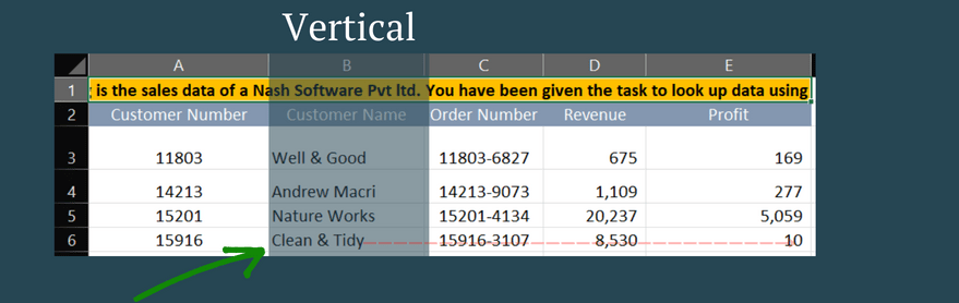
• Firstly, observe the table. The data headers are oriented from left to right.
• Secondly, the value of each header is oriented from top to bottom.
• Thirdly, when we search for data, we know one data point from any of the data headers. For, eg, we might be aware of the customer’s name, and we might want to find out the order number.
• Hence, we look for data vertically, but the related field is horizontal.

Similarly, for an h-lookup, the above explanation would change in the following way.

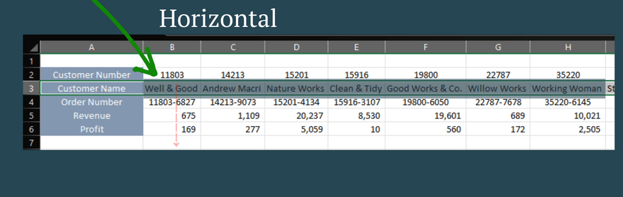
Now, observe in the above image that we search for the customer name from left to right(horizontal). However, we the related data we search vertically.

HLOOKUP in Excel

The HLOOKUP function is a built-in function in Excel that is categorized as a Lookup/Reference Function. HLOOKUP stands for Horizontal Lookup and can retrieve information from a table by searching a row index number range for the matching data and outputting from the corresponding column. HLOOKUP searches for the value in a row. It can be used as a worksheet function (WS) in Microsoft Excel. It is entered as a part of a formula in a cell of the worksheet.

• Syntax: Hlookup formula

 HLOOKUP( lookup_value, table_array, row_index_number, [range_lookup])

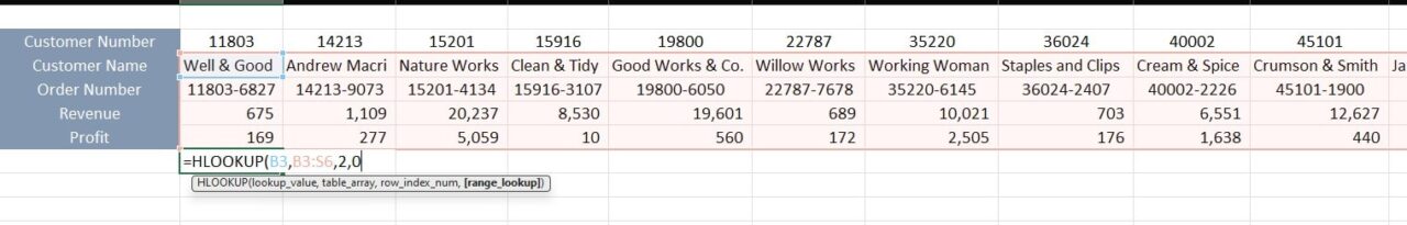
• lookup_value – The value to search for in the first row of the table ( Well& Good)
• table_array – The search area( Just keep in mind to keep the lookup row on the two)

In the example above, I have selected the table array from B3, Its important to keep the look-up value on the top most row. Else this won’t work.

• row_index_number –put the row number where your data search values exist. For, eg; in the above example, I wanted to find the order number, which is row number two. Here the row number is counted from row number 3 to row 6. Hence the order is on row number 4, which is the 2nd row.
• Range lookup select zero if you know the exam value or text. If in case you are not sure about the look-up value, then select 1.
• Range look is false in most of the cases, where we are looking for the exact match.

Applies to:

Excel for Office 365, Excel 2019, Excel 2016, Excel 2013, Excel 2011 for Mac, Excel 2010, Excel 2007, Excel 2003, Excel XP, Excel 2000

HLOOKUP in Excel example

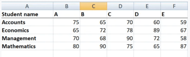
Let us consider the example below. The marks for four subjects for five students are as follows:

Now, if our objective is to fetch the marks of student D in Management, we can use HLOOKUP as follows:

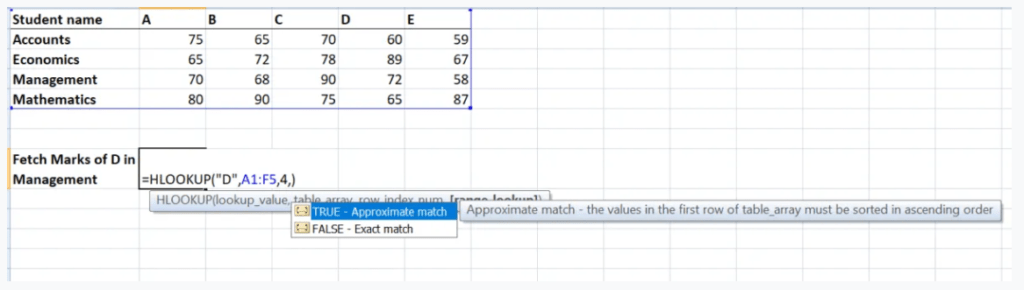
The result would be 72

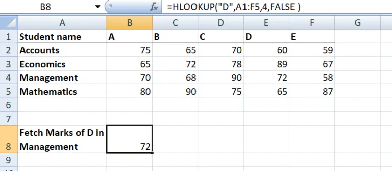
Here, HLOOKUP searches for a particular value in the table and returns an exact or approximate value.

Pros & Cons of H-look up in excel

Pros of H-look up

• Firstly, it’s easy to use and can usually be deployed on horizontally aligned data.
• Secondly, the function can do approximate matches just like v-lookup

Cons of H-look up

• First, the biggest con of the H-look of function is that the look-up row has to be on the top. Now, that might not be the case always, which makes it very rigid to use.

Hlookup in Excel Versus Vlook in excel

Hlookup and Vlookup are both functions in Microsoft Excel that allow users to quickly and easily look up data in a table or range of cells.

The main difference between the two is the direction in which the function searches for data. Hlookup (short for “horizontal lookup”) searches for data in the first row of a table and returns a corresponding value from a specified column. The syntax for Hlookup is: =HLOOKUP(lookup_value, table_array, row_index_num, [range_lookup])

Vlookup (short for “vertical lookup”) searches for data in the first column of a table and returns a corresponding value from a specified row. The syntax for Vlookup is: =VLOOKUP(lookup_value, table_array, col_index_num, [range_lookup])

In summary, Hlookup searches horizontally while Vlookup searches vertically. Also, to use Vlookup, the data should be in a vertical format, and to use Hlookup the data should be in a horizontal format.

Conclusion

Let me be clear here, rarely is data-oriented in a horizontal format. At the same time, data is mainly oriented vertically. Also, the reason for it being the visual easiness. So, data can be seen more easily vertically than horizontally. So, I won’t obsess too much about this function, but neither would I discredit it. Mostly, we use V-lookup in financial modelling.

FAQ’s-hlookup in excel

How to do Hlook up in Excel?

So, to use the hlook up function in excel, first make sure that your data actually qualifies for a hlook-up function. Which, bascially means that, the headers of the data has to be on the rows and the values flow horizontally.

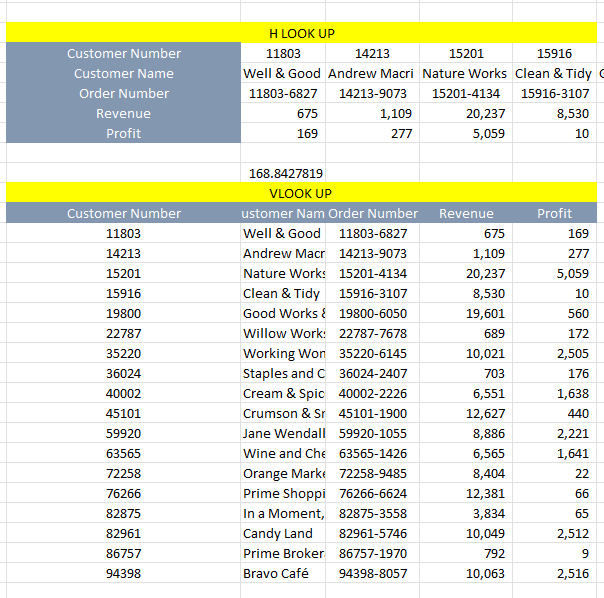
Let’s suppose we want to find the profit related to customer number 11803, then the formula will be as follows:

=HLOOKUP(G6,$F$6:$X$10,5,0)

What is the difference between H lookup and VLOOKUP?

The difference between Hlook up and vlook up function is, that the Hlook looks for data horizontally across coloums, while the Vlook function looks for data vertifically across rows using the col headers. So, below I have shown two data orientation in cases, where we use vlook up or hlook up.