Last updated on October 23rd, 2024 at 04:13 pm
The lookup function in Excel is a powerful tool that enables users to search for specific values within a dataset, providing a convenient way to retrieve related information. With the lookup function, you can effortlessly locate data based on a given criteria, such as a unique identifier or a specific attribute. By using this function, you can streamline your data analysis process and gain insights quickly. Whether you’re searching for sales figures, employee information, or any other data set, the lookup function in Excel simplifies the task by automating the search and retrieval process. Mastering this function is essential for efficient data management and analysis in Excel.
What is the LOOKUP function?
The lookup function is categorised under Microsoft Excel’s lookup and reference functions. This function returns a value from a range (one row or one column) or from an array. It can be used as a worksheet function (WS) in Microsoft Excel. The LOOKUP function can be entered as a part of a formula in a cell of a worksheet. Comparing two columns or rows in financial analysis can be done very easily with the use of the LOOKUP function. This function is designed to handle the simplest cases of vertical and horizontal lookup. The more advanced versions of the LOOKUP function are HLOOKUP and VLOOKUP.
Formula Lookup Function in Excel
There are two forms of the LOOKUP function: vector and array.
- Vector Method:
The vector form of the LOOKUP function will search one row or one column of data for a specified value and then get the data from the same position in another row or column.
Formula =LOOKUP(lookup_value, lookup_vector, [result_vector])
Parameters
- Lookup_value – This is the value that we will be searching for. It can be a logical value of TRUE or FALSE, a reference to a cell, number, or text.
- Lookup_range – A single row or single column of data that is sorted in ascending order. The LOOKUP function searches for a value in this range.
- Result_range – It is a single row or single column of data that is the same size as the lookup_range. The LOOKUP function searches for the value in the lookup_rangeand returns the value from the same position in the result_range. If this parameter is omitted, it will return the first column of data. This is an optional parameter
Returns
The LOOKUP function returns any data type such as a string, numeric, date, etc. If the LOOKUP function cannot find an exact match, it chooses the largest value in the lookup_range that is less than or equal to the value. If the value is smaller than all of the values in the lookup_range, then the LOOKUP function will return #N/A. If the values in the lookup_range are not sorted in ascending order, the LOOKUP function will return the incorrect value.
Applies to
Excel for Office 365, Excel 2019, Excel 2016, Excel 2013, Excel 2011 for Mac, Excel 2010, Excel 2007, Excel 2003, Excel XP, Excel 2000
2. Array Method:
Formula =LOOKUP(lookup_value, array)
Parameters
- Lookup_value – This is the value that we will be searching for. It can be a logical value of TRUE or FALSE, a reference to a cell, number, or text.
- Array – A range of cells that contains text, numbers, or logical values that we want to compare with the lookup_value.
How to use the LOOKUP function in Excel?
Example 1:
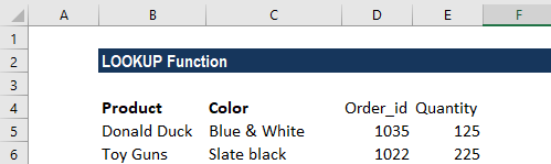
Assume we are given a list of products, colour, order_id, and quantity. We want a dashboard where we put the product and then we instantly get the quantity.
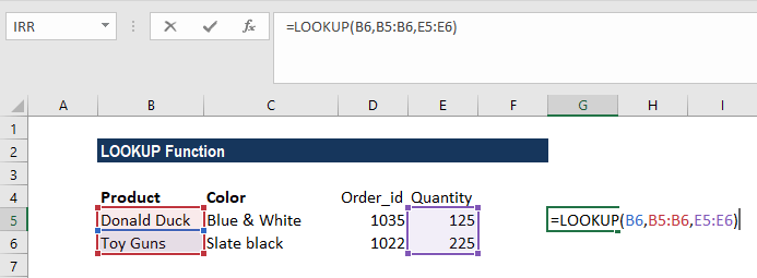
The formula to use will be:
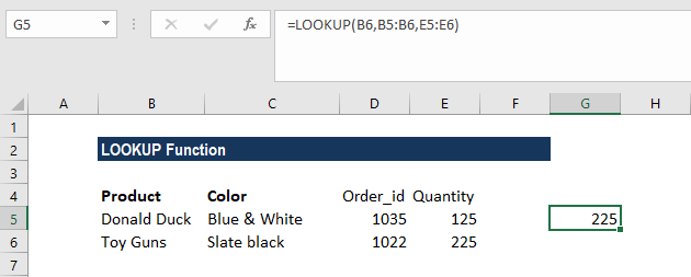
The result we get is:
Example 2:
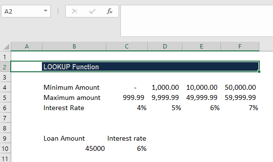
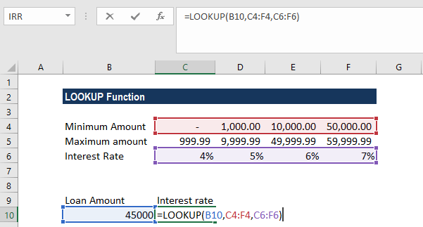
Suppose we are in the business of giving loans and we offer different interest rates based on the amount borrowed. We are given the data below:
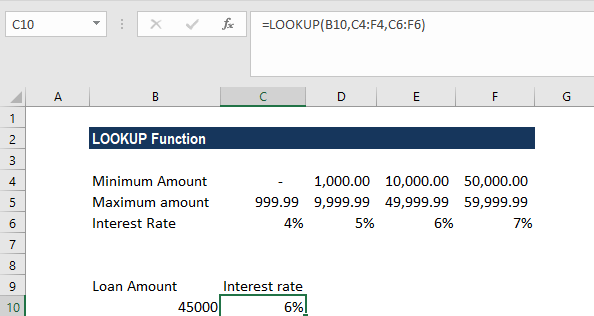
The formula to use will be:
We will get the following result:
Advantages of Using Lookup Function
The lookup function in Excel offers several advantages that make it an indispensable tool for data analysis and management. Here are some key advantages of using the lookup function:
- Efficient Data Retrieval: The lookup function allows you to quickly locate and retrieve specific data from large datasets. Instead of manually searching through rows and columns, the function automates the process, saving you time and effort. This efficiency is especially valuable when dealing with extensive databases or when you need to find information regularly.
- Accurate Results: By using the lookup function, you can ensure accurate results when searching for data. The function performs precise matches based on the specified criteria, eliminating the chances of human error or oversight. This accuracy is crucial for maintaining data integrity and making informed decisions based on reliable information.
- Flexibility in Data Analysis: The lookup function provides flexibility in data analysis by allowing you to perform various types of searches. For instance, you can perform exact matches, approximate matches, or even find the closest match to a given value. This versatility enables you to adapt the function to different scenarios and tailor your analysis to specific requirements.
- Integration with Other Functions: The lookup function seamlessly integrates with other Excel functions, expanding its capabilities and enhancing data analysis possibilities. You can combine the lookup function with mathematical functions, logical functions, or even with conditional formatting, allowing you to perform complex calculations and evaluations on retrieved data.
- Handling Changing Data: One significant advantage of the lookup function is its ability to handle changing data dynamically. If your dataset undergoes modifications or updates, the lookup function can automatically adjust and retrieve the updated information based on the specified criteria. This feature ensures that your analysis remains up to date, even in a dynamic data environment.
Related
A CFA charterholder with hands-on experience across investment analysis and finance education. At MentorMeCareers, he writes and reviews content on CFA, financial modeling, and investment banking careers — grounded in real market data rather than generic advice, and shaped by what actually helps candidates and professionals succeed.