Last updated on October 23rd, 2024 at 02:12 pm
CAPM full form stands for capital asset pricing model, is a formula to calculate the expected return on equity for a business. However, I must clarify this that it is just a model. Which means, CAPM is a model to estimate the cost of equity for a business or stock.
So let me get started with discussing in detail about CAPM Full form, uses and examples.
All About CAPM Full Form And More

What is the CAPM Full form
The CAPM full form is the Capital Asset Pricing Model, which is a market model made to investigate the link between risk and necessary rates of return on assets held in well-diversified holdings.
Now that might sound like a mouth full. However, CAPM (full form- Capital asset pricing model) is just to calculate, what is the return you should be expecting from a security or a business.
For eg; Let’s suppose, I tell you that there is a buisiness can give INR 40 Lacs every year for 5 years. For which, you will have to invest 10 Lacs INR. Then the next question would be, what is the present value of these future cash flows.
While we are aware that Present value = Future value of cash flows/ (1+r), where the interesting this is the r. That r in question, is what I can estimate two methods
- Opportunity cost- Your highest return generated on your current money
- Second, is CAPM.
Illustration for CAPM Full Form
The Capital Asset Pricing Model (CAPM) establishes a linear link between a security’s necessary rate of return (Ri) and its structural or undiversifiable risk, as measured by beta. The market volatility is not avoidable by diversification is the measure of the risk of an asset, which is assessed mostly by the beta coefficient of such security.
Assumptions in CAPM(Full form Capital asset pricing model)
- All clients are a single-period anticipated utility of ultimate wealth maximizers who pick between various portfolios depending on projected return and statistical significance of portfolios.
- At a risk-free rate of interest, every investor can borrow or lend a limitless amount.
- Investors all have the same objectives (that is, capitalists have identical estimations of the predicted values, discrepancies, and covariances of tax return among all assets).
- There are no trade expenses, and all assets are completely divisible and tradable at the prevailing price.
- There are no fees or charges.
- Every capitalist is a price taker (that is, all asset investors consider that their buying and sale activity will not influence the price of the stock).
- All of the assets’ amounts are predetermined.
CAPM Full form Formula
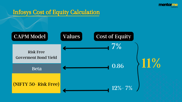
The needed return on a security, as per the Capital Asset Pricing Model (CAPM) method, is provided by the equation:
Ri = Rf + βi ( Rm — Rf )
Where,
Ri= The required return rate on a security, or the cost of equity, is referred to as Ri.
Rf= The risk-free return rate (Rf) is a rate of return that is calculated without taking any risks.
Î2i = Security i’s Beta
Rm = It is the market portfolio’s rate of return.
Rm- rf= Market risk premiun
Applications of CAPM Full form
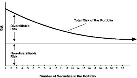
So before, you can actually understand the applications you need to understand that there two types of risks in any investment. For example; if you invest in real estate then you are taking two risks.
- General risk of the real estate market risk, also called as systematic risk
- Specific risk related to your target property, un-systematic risk
Now, if I asked you a question. By investing in real estate can you eliminate the risk of real estate market itself? Secondly, can you eliminate the property specific risk?
Now, hopefully your answer to the first question should be, “No”, and the answer to the second should ” Yes”. However, how can you? It’s simple, instead of investing in one large property, invest in 4 smaller properties of diiferent types and different locations. The answer I gave just now is theoritcal, so don’t go and buy yet. However, this investment can actually be done in practical by investing in REITS(Real estate investment trusts).
Hence, the next part where I am talking about Security market line, is exactly talking about the undersized risk of real estate in general and the cost of equity or return we calculated in CAPM Full form illustration. Also, remember the undiversified risk, is also called as beta.
Analysis of the Security Market Line (SML)- CAPM
The Security Market Line is a graphical representation of the link between the necessary return on capital (ke) and the non-diversifiable risk (beta) of an asset (SML). This also means, that you can keep on adding more types of stocks, untill the diversifiable risk is reduced to almost zero,
At the same time, remember that reducing the diversifiable risk will also keep on reducing the overall returns.
The Security Market Line, also known as SML, is a tradeoff between projected return and security risk (beta risk) compared to the market portfolio used by the CAPM model. Any individual security’s projected yield and beta should sit on the SML under equilibrium conditions. Because all securities are supposed to chart all along SML, again, when the beta of the asset is known, the line gives a clear means to forecast the future (required) return of the security.
SML and CML
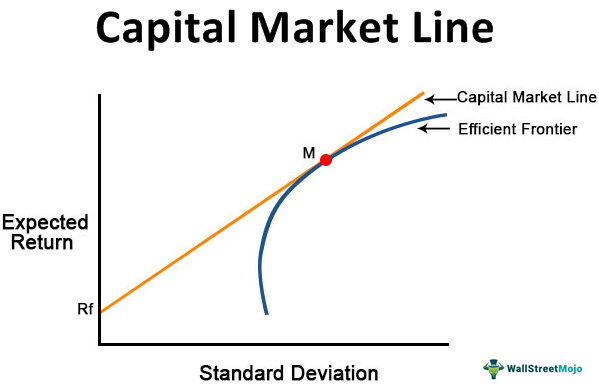
The CML plots the returns expectation of an optimal portfolio (those that include both the market and a risk-free investment). It works as a function of asset standard deviation. Which is that Standard deviation is a reasonable way to estimate risk for effective portfolio diversification that are prospects for an investor’s total portfolio.
In a nutshell, all we are trying to find is a point in the capital market line, where the combination of risk free security + the portfolio gives us the lowest possible risk for the highest amount of returns.
The security market line (SML) serves as a standard against the measurements of investment performance. The SML calculates the required rate of return to pay shareholders for both risk and the value of the investment. It is further based on the risk of an asset as defined by its beta. Because of SML, it is a visual depiction of the expected profit relationship, ‘fairly priced’ assets plot precisely on it; their projected rewards are proportional to their risk. All assets must be in market equilibrium on the SML, given the assumption we stated at the beginning of this article.
If a stock is thought to be a good purchase or under-priced, this will yield a higher projected return than the SML’s fair return. Undervalued equities, on the other hand, the plot just above SML because their projected returns are higher than those predicted by the CAPM. Stocks that are overvalued are shown below the SML.
Capital Asset Pricing Model Empirical Tests (CAPM)
Empirical tests should be employed to verify the Capital Asset Pricing Model (CAPM) because it was built based on a set of unreasonable assumptions.
The first test checks for historical beta stability. If a stock’s betas have been steady in the past, its historical beta is likely to be a strong indicator for some of its ex-ante, or expected, beta. Individual stock betas are not strong predictors of future risk, according to empirical research, but portfolio betas of 10 or more randomly chosen stocks are relatively steady, implying that previous portfolio betas are decent predictors of future portfolio variance.
The inclination of the SML is useful for the 2nd type of test. The CAPM asserts that the needed average return and beta of security have a linear connection, as we’ve seen. The vertical axis intercept for a commodity (or portfolio) with beta = 1.0 should be RF. The necessary dividend yield for a commodity (or portfolio) with the help of beta = 1.0 must be Rm, the required return rate on the market for the graphic of SML. Several academics have attempted to validate the CAPM model’s validity by computing betas and realized rates of return, putting these values on graphs. Then checking whether the intercept equals RF, the linear regression is straight, and the SML crosses via the point of b = 1.0, Rm. Evidence suggests that realized profits and market volatility have a more-or-less linear connection, but the slope is lower than the expectations. The irrelevance of residual risk indicated throughout the CAPM model might be questioned. It is the work of tests attempting to quantify the relative impact of the marketplace and business risk that do not give decisive findings.
When it comes to portfolios, data appears to confirm the CAPM model, but when it comes to individual equities, the data is less persuasive.
Nonetheless, the CAPM is a sensible method to look at return and risk as long as one understands the CAPM’s limits when being used in reality.
CAPM-Capital Asset Pricing Model’s Recent Developments
Since its introduction in the 1960s, several scholars have chosen to expand and enhance the conventional Capital Asset Pricing Model. The pricing models of assets have undergone significant changes to improve their realism.
The model with Three Factors
The implied volatility estimation, or the difference between both the rate of return and the risk-free rate of interest, is a crucial assumption in CAPM. Fama and French developed and suggested the Three-Factor Model in response to mounting scientific findings that the CAPM failed to adequately explain actual returns. When designing the conventional CAPM, Fama and French included two factors: market cap and book-to-market valuation, with the goal of better explaining portfolio results. They discovered a correlation between the company’s book-to-market proportion and scale in 1995, to calculate the stock’s return. The verification of the Three-Factor Model has more predictive value than that of the one-factor CAPM after repeatable experiments. It indicates that the key advantage of this system is that it incorporates the firm’s size and worth, and the CAPM’s market risk component.

The model with Five Factors
Following the development of the 3-factor model, Fama and French proceeded to construct the Five-Factor model, which further expanded on this idea. The creation of this model takes into account not only the firm’s size and worth but also the market risk element, as well as the profit of the stock and investing patterns in typical stock returns. The five-factor model’s empirical tests attempt to explain annual returns on portfolios constructed to create big scale, profit, and investment spreads. The value of the prior three-factor model is rendered obsolete by the addition of dividend payout ratio elements.
Arbitrage Pricing Theory (APT)
Arbitrage Pricing Theory (APT) With the premise that various equities would have varying sensitivity to different market conditions, the Arbitrage Pricing Theory tries to alleviate the constraints of the one-factor CAPM. The APT assumes that an asset is influenced by a variety of macroeconomic factors, such as inflation, currency rates, market indices, interest rate movements, and market attitudes, to mention a few. Simply put, not all investments or equities will respond the same way to the same parameter all of the time, necessitating the consideration of multi factors and sensitivities.
CAPM with no beta
The Zero-Beta CAPM, created by Black around 1972, demonstrated that the outcomes of CAPM do not necessitate a risk-free asset with constant returns in all states of nature. A portfolio designed without systematic risk is known as a zero-beta portfolio. The zero-beta CAPM assumes that beta has always been the accurate measure of the risk and also that the model is still linear. It implies that the portfolio’s value is unaffected by market fluctuations. In a zero-beta investment, yield is just like the risk-free rate since there is no systematic risk. As a result, the return on investment with zero betas will be lowered, and without the market’s volatility revealed, the portfolio would be unable to gain from prospective market periods of growth.
Inter-Temporal CAPM
The one-time period assumptions of the standard CAPM have been given relaxation in ICAPM. It is believed that ICAPM investors are concerned primarily with the end-of-period payback, as well as the opportunity to consume or put the money in this payoff, whereas ordinary CAPM investors are concerned with the worth of their holdings after the current cycle. The Inter-temporal CAPM assumes a perfect market with no costs or taxes, limited responsibility for all assets, investors believing their decisions do not influence market pricing, and the marketplace is always in balance, among other assumptions. The ICAPM transcends the CAPM towards a more dynamic setting, with findings that are almost identical to those of the APT. The distinction between ICAPM and APT, though, would be that the ICAPM may assess risks based on asset attributes.
CAPM’s Downside (Downside BETA)
Another extension of the CAPM is the Downside BETA or Downside-CAPM. This idea has a long history. In the typical CAPM, beta employment is for calculation of the expected rate of return of a commodity. The potential loss of an asset, or the danger of loss, is measured using downside beta. Investors may want to think about building their portfolios so that the downside beta is as low as possible. It is to assure that they can preserve the value in the event of a market downturn.
CAPM Revision
This model is an extension of the traditional Capital Asset Pricing Model, which takes into account economic, operating, and economic constraints. It focuses on both systematic risk and unsystematic risk, as well as historical and estimated data, to produce a more accurate return projection. They compared R-CAPM to the standard CAPM, the Downside CAPM, and the Adjusted-CAPM while evaluating this model and discovered that the metrics of anticipated return rate for R-CAPM and the alternate of CAPMs differed significantly.
CAPM consumption (Co-CAPM)
The CAPM for Consumption is an enhancement to the basic CAPM. The fluctuation of the premiums with growth momentum is used to calculate Co-CAPM quantity market risk. As a result, the Co-CAPM indicates how much more the entire share market changes as a result of rising consumption. Although this model is claimed to be the greatest theoretical model, the Co-core CAPM’s relationship between both consumption and market return cannot be maintained. The Co-CAPM is more commonly employed in academia since it encompasses a wide range of wealth, not only stock market wealth, and allows for the analysis of return variations over time.
CAPM Reward (Reward-BETA)
Graham Bornholt remarked in 2006 that to maximize the profit, a better approach to assess projected returns to the share market. He created the Reward-BETA CAPM with this in mind. The assumptions behind this model are congruent with the Arbitrage Theory, which divides stock returns into two categories: anticipated and unforeseen stock returns.
Related Articles
A CFA charterholder with hands-on experience across investment analysis and finance education. At MentorMeCareers, he writes and reviews content on CFA, financial modeling, and investment banking careers — grounded in real market data rather than generic advice, and shaped by what actually helps candidates and professionals succeed.